Chapter 3 Pre-processing of bulk RNA-seq data
In this chapter, we will align RNA-seq data, check the data quality, quantify gene expression and handle batch effects across samples. To run the RIMA preprocess modules, in execution.yaml, set preprocess_individual and preprocess_cohort to true. The individual run of the preprocess module includes read alignment, quality checks and gene quantification. The cohort run of the preprocess module will merge data from all samples to produce cohort level reports for alignment, quality metrics and gene quantification. The cohort run will also conduct batch effect removal.
## execution.yaml ##
preprocess_individual: true
preprocess_cohort: true
3.1 Read Alignment
Align reads with STAR
STAR is one of the most common tools used for bulk RNA-seq data alignment to generate transcriptome BAM or genomic BAM output, which can be downloaded at here. A tutorial for STAR is available here.
When using STAR, the first step is to create a genome index. In our RIMA pipeline, we download the human genome (hg38) STAR index from Genomic Data Commons (GDC) .Let’s use sample SRR8281218 as an example.
RIMA runs STAR using the following command structure:
      STAR --runThreadN 4 --genomeDir ./ref_files/v22
        --outReadsUnmapped None
        --chimSegmentMin 12
        --chimJunctionOverhangMin 12
        --chimOutJunctionFormat 1
        --alignSJDBoverhangMin 10
        --alignMatesGapMax 1000000
        --alignIntronMax 1000000
        --alignSJstitchMismatchNmax 5 -1 5 5
        --outSAMstrandField intronMotif
        --outSAMunmapped Within
        --outSAMtype BAM Unsorted
        --readFilesIn {input}
        --chimMultimapScoreRange 10
        --chimMultimapNmax 10
        --chimNonchimScoreDropMin 10
        --peOverlapNbasesMin 12
        --peOverlapMMp 0.1
        --genomeLoad NoSharedMemory
        --outSAMheaderHD @HD VN:1.4
        --outFileNamePrefix {params.prefix}
        --quantMode TranscriptomeSAM
RIMA renames the read aligment outputs according to sample id.
analysis/star/SRR8281218/SRR8281218.sorted.bam
analysis/star/SRR8281218/SRR8281218.transcriptome.bam
analysis/star/SRR8281218/SRR8281218.Chimeric.out.junction
analysis/star/SRR8281218/SRR8281218.Log.final.out
RIMA also uses samtools to generate statistics from the alignment BAM file:
samtools stats analysis/star/SRR828121/SRR8281218.sorted.bam | grep ^SN | cut -f 2- > analysis/star/SRR8281218/SRR8281218.sorted.bam.stat.txtMerging the STAR alignment reports
After the individual alignment runs of each sample, RIMA will merge the alignment reports from all samples to generate a file named STAR_Align_Report.csv. Below is an example of merged output:
STAR,SRR8281218,SRR8281219,SRR8281226,SRR8281236,SRR8281230,SRR8281233,SRR8281244,SRR8281245,SRR8281243,SRR8281251,SRR8281238,SRR8281250
Number_of_input_reads,31058961,30244952,30144822,30214970,30219317,30294851,30233324,30188854,30267936,30155916,30238326,30205607
Average_input_read_length,200,200,200,200,200,200,200,200,200,200,200,200
Uniquely_mapped_reads_number,29396418,28842972,27785223,28625526,28552141,29084522,29172831,28527204,28611921,28526789,26648329,28820905
Uniquely_mapped_reads_%,94.65%,95.36%,92.17%,94.74%,94.48%,96.00%,96.49%,94.50%,94.53%,94.60%,88.13%,95.42%
Average_mapped_length,198.82,198.69,198.65,198.64,198.64,198.54,198.64,198.54,198.66,198.64,198.71,198.62
Number_of_splices:_Total,14076881,16545751,18439209,15091999,14432943,15290737,16116559,18614840,14065847,13967615,9829323,14650425
Number_of_splices:_Annotated_(sjdb),14043726,16506835,18399706,15050436,14388389,15246382,16073843,18570667,14031241,13930154,9801357,14610503
Number_of_splices:_GT/AG,13944521,16380126,18275777,14941222,14287227,15142625,15961566,18425036,13939221,13836881,9738054,14508837
Number_of_splices:_GC/AG,106767,133082,130042,118569,116171,114096,121618,134112,97534,102169,69796,112736
Number_of_splices:_AT/AC,11811,14116,14898,13200,12486,11590,12575,12673,11867,11783,7031,13252
Number_of_splices:_Non-canonical,13782,18427,18492,19008,17059,22426,20800,43019,17225,16782,14442,15600
Mismatch_rate_per_base_%,0.20%,0.18%,0.17%,0.18%,0.19%,0.18%,0.17%,0.19%,0.19%,0.19%,0.18%,0.17%
Deletion_rate_per_base,0.01%,0.00%,0.00%,0.01%,0.00%,0.01%,0.00%,0.00%,0.01%,0.01%,0.01%,0.00%
Deletion_average_length,1.29,1.29,1.26,1.29,1.28,1.21,1.29,1.26,1.22,1.22,1.12,1.23
Insertion_rate_per_base,0.01%,0.01%,0.01%,0.01%,0.01%,0.01%,0.01%,0.01%,0.01%,0.01%,0.01%,0.01%
Insertion_average_length,1.40,1.43,1.42,1.44,1.44,1.45,1.42,1.41,1.41,1.40,1.37,1.40
Number_of_reads_mapped_to_multiple_loci,1331220,1119545,2078090,1280274,1347073,901525,766599,1332933,1325151,1337251,3322861,1103343
%_of_reads_mapped_to_multiple_loci,4.29%,3.70%,6.89%,4.24%,4.46%,2.98%,2.54%,4.42%,4.38%,4.43%,10.99%,3.65%
Number_of_reads_mapped_to_too_many_loci,9535,10773,11999,12262,15652,9758,8344,10240,8594,10179,9217,8381
%_of_reads_mapped_to_too_many_loci,0.03%,0.04%,0.04%,0.04%,0.05%,0.03%,0.03%,0.03%,0.03%,0.03%,0.03%,0.03%
%_of_reads_unmapped:_too_many_mismatches,0.08%,0.09%,0.12%,0.13%,0.13%,0.14%,0.10%,0.24%,0.13%,0.12%,0.11%,0.09%
%_of_reads_unmapped:_too_short,0.92%,0.76%,0.73%,0.81%,0.83%,0.81%,0.80%,0.77%,0.90%,0.77%,0.70%,0.78%
%_of_reads_unmapped:_other,0.04%,0.04%,0.05%,0.04%,0.05%,0.03%,0.04%,0.04%,0.03%,0.05%,0.04%,0.04%
Number_of_chimeric_reads,592271,594198,549596,631747,635307,717293,631225,666748,637640,622475,600743,636839
%_of_chimeric_reads,1.91%,1.96%,1.82%,2.09%,2.10%,2.37%,2.09%,2.21%,2.11%,2.06%,1.99%,2.11%
3.2 Quality Control
Downsampling alignment BAMs
RseQC is a standard tool for checking the quality of read alignments, providing the principal measurements of RNA-seq data quality. An RseQC tutorial is available here.
To reduce running time, we first sub-sample sorted BAM files to be used by RseQC to assess alignment quality. If parameter ‘rseqc_ref’ is set to ‘house_keeping’, RIMA will extract alignments of house keeping genes for the sub-sample.
## Example of subsampling 50% of input alignments
samtools view -s 0.5 -b analysis/star/SRR8281218/SRR8281218.sorted.bam  > analysis/star/SRR8281218/SRR8281218_downsampling.bam

# Extract the alignment of housekeeping genes.
bedtools intersect -a analysis/star/SRR8281218/SRR8281218_downsampling.bam  -b ./ref_files/housekeeping_refseqGenes.bed > analysis/star/SRR8281218/SRR8281218_downsampling_housekeeping.bam

# index BAM
samtools index analysis/star/SRR8281218/SRR8281218_downsampling_housekeeping.bam  > analysis/star/SRR8281218/SRR8281218_downsampling_housekeeping.bam.bai
RseQC Quality metrics
- Transcript integrity number (TIN) is the most widely used measure of RNA integrity, which is the percentage of transcripts that have uniform read coverage across the genome. RseQC calculates the TIN of each transcript and reports mean TIN, median TIN and standard deviation for all transcripts in a sample. The median TIN score (medTIN) across all transcripts is commonly used to indicate the RNA integrity of each sample.
- Read distribution summarizes the fraction of reads aligned into different genomic regions, such as exon and intron regions.
- Gene body coverage shows the RNA-seq read coverage over the gene body.
Low quality samples have low alignment fractions, low integrity (median TIN) and/or abnormal read distributions and should be removed in downstream analysis.
Merge quality metrics
RIMA will also merge quality metrics for all samples. Below are examples of the merged outputs for TIN score tin_score_summary.txt and read distribution read_distrib.matrix.tab:
##tin_score_summary.txt##
Bam_file    TIN(mean)   TIN(median) TIN(stdev)
SRR8281218_downsampling_housekeeping.bam    72.59011823410742   76.61544321066245   15.70457852012789
SRR8281219_downsampling_housekeeping.bam    74.53459359515176   78.36139111185804   14.862696392336295
SRR8281226_downsampling_housekeeping.bam    72.12569765806015   76.04482057429738   15.150628049210777
SRR8281236_downsampling_housekeeping.bam    75.10959004809101   79.0211107295296    14.112536675463657
SRR8281230_downsampling_housekeeping.bam    74.95210786264646   78.18898561188249   14.084506430648968
SRR8281233_downsampling_housekeeping.bam    71.91235332638948   76.36385765230236   16.193874225558574
SRR8281244_downsampling_housekeeping.bam    72.42514699067206   76.9844608754321    16.270160903196263
SRR8281245_downsampling_housekeeping.bam    72.16726184355547   76.41674529483181   15.380595156507917
SRR8281243_downsampling_housekeeping.bam    71.56229409539716   74.7019940049169    13.711275796768888
SRR8281251_downsampling_housekeeping.bam    73.02855865353006   77.30010010150008   14.902687257461483
SRR8281238_downsampling_housekeeping.bam    66.23444336304713   70.08838336433544   17.437545601110816
SRR8281250_downsampling_housekeeping.bam    75.25874145796432   78.83524471249612   14.125154826821316

##read_distrib.matrix.tab##
Feature SRR8281218  SRR8281219  SRR8281226  SRR8281236  SRR8281230  SRR8281233  SRR8281244  SRR8281245  SRR8281243  SRR8281251  SRR82
81238   SRR8281250
TES_down_1kb    0.00    0.00    0.00    0.00    0.00    0.00    0.00    0.00    0.00    0.00    0.00    0.00
TSS_up_1kb  0.00    0.00    0.00    0.00    0.00    0.00    0.00    0.00    0.00    0.00    0.00    0.00
TSS_up_5kb  0.00    0.00    0.00    0.00    0.00    0.00    0.00    0.00    0.00    0.00    0.00    0.00
Introns 0.05    0.05    0.03    0.06    0.08    0.06    0.05    0.04    0.04    0.04    0.04    0.04
TES_down_5kb    0.00    0.00    0.00    0.00    0.00    0.00    0.00    0.00    0.00    0.00    0.00    0.00
CDS_Exons   0.80    0.81    0.85    0.79    0.77    0.79    0.79    0.83    0.80    0.80    0.81    0.80
3'UTR_Exons 0.12    0.11    0.08    0.12    0.11    0.12    0.11    0.09    0.12    0.11    0.11    0.12
TES_down_10kb   0.00    0.00    0.00    0.00    0.00    0.00    0.00    0.00    0.00    0.00    0.00    0.00
5'UTR_Exons 0.04    0.04    0.04    0.03    0.03    0.03    0.04    0.04    0.03    0.04    0.04    0.04
TSS_up_10kb 0.00    0.00    0.00    0.00    0.00    0.00    0.00    0.00    0.00    0.00    0.00    0.00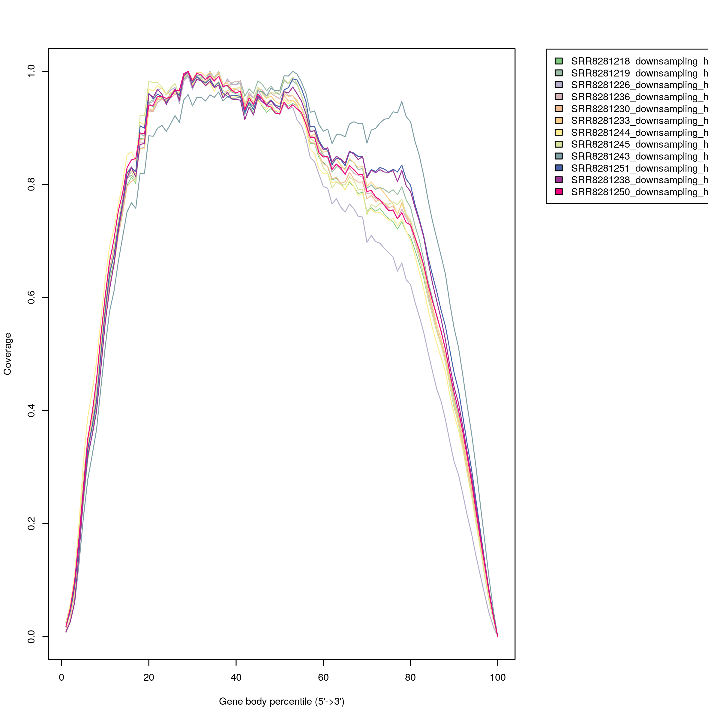
Figure 3.1: Gene Body Coverage Curves
3.3 Gene quantification
After the alignment of sequencing reads and quality checks, we quantify the gene or transcript expression from the BAM files.Both Salmon and RSEM are widely used for gene quantification. Salmon conducts fast transcript-level quantification, and RSEM performs both gene-level and transcript-level quantification. Salmon is usually faster and less memory-consuming than RSEM. RSEM generates transcripts per million (TPM), reads per kilobase of exon model (transcript) per million mapped reads (RPKM) and fragments per kilobase of exon model (transcript) per million mapped reads (FPKM) expression. Salmon provides TPMs as a part of its output. All three measures (TPM, RPKM, FPKM) are normalization methods that account for both sequencing depth and gene lengths. (Longer transcripts will have more reads.) TPM is currently thought to be the best method to normalize gene counts. HTSeq quantifies gene expression according to mapped read counts. Both normalized gene expression and raw read counts can be used for differential expression analysis.
RIMA uses Salmon for gene quantification. The transcriptome alignment result from STAR is used as the Salmon input:
salmon quant -t ./ref_files/salmon_gdc_index/gencode.v22.ts.fa -l A -a analysis/star/SRR8281218/SRR8281218.transcriptome.bam -o analysis/salmon/SRR8281218The following is an example of an output file from Salmon
Name    Length  EffectiveLength TPM NumReads
ENST00000456328.2   1657    1474.085    0.000000    0.000
ENST00000450305.2   632 449.595 0.000000    0.000
ENST00000488147.1   1351    1168.085    7.412619    139.959
ENST00000619216.1   68  69.000  0.000000    0.000
ENST00000473358.1   712 529.382 0.000000    0.000
ENST00000469289.1   535 353.431 0.000000    0.000
ENST00000607096.1   138 16.202  0.000000    0.000
RIMA then uses ‘tximport’ from the DESeq2 R package to combine a cohort’s gene level TPMs into a summary file:
## First 10 rows of merge TPMs ##
SRR8281218,SRR8281219,SRR8281226,SRR8281236,SRR8281233,SRR8281230,SRR8281244,SRR8281245,SRR8281243,SRR8281238,SRR8281251,SRR8281250
5_8S_rRNA,0,0,0,0,0,0,0,0,0,0,0,0
5S_rRNA,0,0,0,0,0,0,0,0,0,0,0,0
7SK,0,0.75,1,5.864,5.667,5,1.961,2.67,10.47,3.531,5,2.981
A1BG,98.378,248.265,222.032,106.318,159.868,262.034,210.18,157.196,83.865,137.558,130.693,193.207
A1BG-AS1,82.273,252.763,70.572,80.758,100.73,297.316,119.662,145.835,66.107,59.74,90.452,168.508
A1CF,2,2,0,3,0,0,0,0,1,2,1,196
A2M,14326.273,9018.603,27465.295,22061.332,31646.181,4559.962,14865.119,20065.994,30592.578,19598.148,12355.795,7203.953
A2M-AS1,59.728,6.397,12.704,36.667,52.819,4.038,24.881,13.006,34.423,23.852,6.206,25.047
A2ML1,180.001,0,17,42,83,55,93,0,12,10,9,763.998
A2ML1-AS1,0,0,0,0,0,0,0,0,0,3.506,0,0
3.4 Batch effect removal
Batch effects across samples are easily overlooked but worth considering for immunotherapy cohort studies. Batch effects are usually caused by unbalanced experimental design and confound the estimation of group differences. For example, samples processed at different facilities may have sequencing differences that are not due to actual biological differences in the samples themselves. To avoid confounding actual biological variation with the effects of experimental design, limma and Combat are common approaches to correct batch effects. Limma uses a two-way ANOVA approach. Combat uses an empirical Bayes approach, which is critical for small batches to avoid over-correction. For large batches, both methods should be similar. The sva R package integrates both methods for batch effect correction. Principal components analysis (PCA) or unsupervised clustering before and after batch effect removal is an excellent way to validate that a batch effect has been removed.
To evaluate if your samples have a batch effect, RIMA will generate PCA plots of gene expression data before and after batch effect removal by limma. To utilize this feature, modify the “batch” parameter in the config.yaml file for your run.
Example of PCA before and after batch correction using limma. (Note: No batch effect was found in the original data used for this tutorial. To generate this diagram, we added a ‘syn_batch’ column to the metasheet for demonstration purposes.)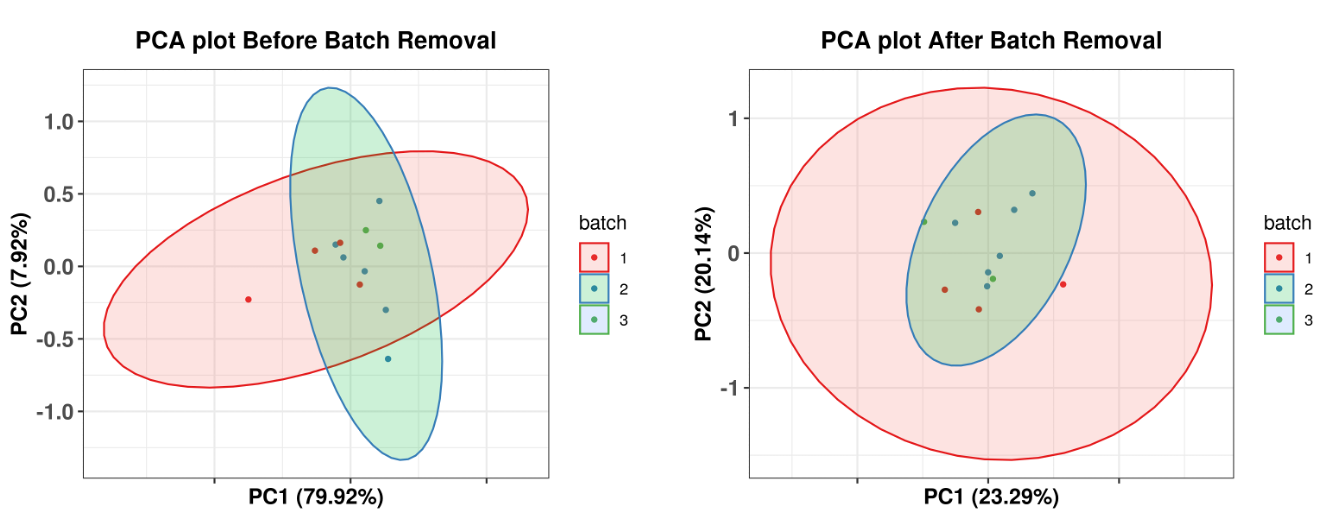
Figure 3.2: Before(left) and after(right) batch correction with Limma
3.5 Video demo of RIMA