Chapter 6 Immune repertoire
A key part of immune specific analysis is assessing the nature of the T and B cells that make up the tumor microenvironment. This assessment includes, but is not limited to, measures such as receptor diversity and clonality.
Once tumors are infiltrated with T cells and B cells, the T cells and B cells are activated if their receptors – TCRs and BCRs, respectively – recognize and bind to tumor-associated antigens. TCRs and BCRs are highly diverse to allow different T and B cells to recognize different pathogens or tumor-associated antigens. Part of the diversity of TCRs and BCRs is due to V(D)J recombination which mixes and matches different V, D and J segments of the genome in order to produce a wide variety of receptors.
Complementary-determining region 3 (CDR3) is a highly variable region of both TCRs and BCRs that is central to the antigen binding site of these receptors. V(D)J junctional sequence assembly is a major source of TCR/BCR CDR3 diversity. Immune repertoire profiling (characterizing the CDR3 sequences of TCRs and BCRs in a tumor sample) is essential for quantifying T/B cell diversity and clonality. These measures, in turn, are important tumor immune characteristics and key indicators of immunotherapy response.
Currently, newly-emerging immune sequencing techniques, such as TCR-seq and BCR-seq, have been designed to sequence T and B cell receptors through quantitative PCR (qPCR). However, TCR-seq and BCR-seq are costly and not always available for particular datasets. To overcome this difficulty, Tcr Receptor Utilities for Solid Tissue (TRUST) has been developed to infer the immune repertoire from bulk RNA-seq reads. V(D)J recombination results in sequences that do not align to genome references. TRUST combines reads that align to the V, D or J regions of the reference genome with sequences that do not align to the host genome to infer de novo assembled CDR3 sequences.
TRUST provides an overview of the immune repertoire of tumors, including CDR3 sequence length and the frequency of various V genes, J genes, and VJ pairs for different chains in the TCR and BCR. For cohort analysis, some basic metrics for TCRs and BCRs across samples could be computed to relate immune repertoire characteristics to specific phenotypes, including the fraction of reads mapped to TCR/BCR, the number of TCR/BCR unique clonotypes of CDR3 sequences, TCR/BCR diversity, and clonality. Since activated B cells undergo somatic hyper-mutation, antibody production, and Immunoglobulin (Ig) class switches during B cell maturation, TRUST also calculates the somatic hypermutation (SHM) rate for BCRs. In addition, TRUST predicts Ig isotypes for BCRs, which allows for quantification of the Ig compositions representing different maturation statuses (IGHM, IGHD, IGHG3, IGHG1, IGHA1, IGHG2, IGHG4, IGHA2, IGHE) and generation of an Ig class switches network. Taken together, the immune repertoire analysis quantifies the T/B cell population at both the individual and cohort levels, enabling one to characterize dynamic evolution in the TME via the diversity and clonal expansion of tumor-infiltrating T cells or B cells.
RIMA currently uses the fourth version of TRUST, TRUST4.
6.1 TRUST4
Example Command:
./run-trust4 -b example.bam -f hg38_bcrtcr.fa --ref human_IMGT+C.faThe above command utilizes hg3_bcrtcr.fa (a fasta file containing the coordinates and sequences of V/D/J/C genes) and human_IMGT+C.fa (a V/D/J/C gene reference file from the IMGT database), and produces a simple report (example_report.tsv). This report contains a list of assembled clonotypes from example.bam with the following fields: “read_count, frequency(proportion of read_count), CDR3_dna, CDR3_amino_acids, V, D, J, C, consensus_id, consensus_id_full_length”. These fields contain the abundance, CDR3 sequence (nucleotides and amino acids), gene segment usage and identifier for each clonotype.
6.1.1 TRUST4 output
In the example codes below, we use one sample to illustrate how RIMA processes the results from TRUST4. RIMA directly adds the sample ID to the TRUST4 output file. This step makes it easier to combine all of individual sample results in the subsequent analysis. In the last section, we describe the cohort level report.
6.2 BCR cluster calculation
Activation of B cells leads to somatic hypermutation (SHM). As B cells proliferate, random mutations are generated at a high rate in the V-region sequence. Favorable mutations lead to better antigen binding and are selected for survival as the B cells continue to proliferate. BCR clustering is used to identify BCRs from the same lineage. The clusters can then be used to estimate somatic hypermutation rate (described later in this chapter).
library(dplyr)

#load processed function
source("TRUST4/trust4_metric_functions.R")

# read the individual sample result from RIMA
cdr3 <- read.table(file = "TRUST4/SRR8281233_cdr3.out.processed.txt", sep = "\t", header = TRUE, stringsAsFactors = FALSE)

#filter out count of cdr ==0 and add the phenotype info for downstream comparison
#This SRR8281233 smaple is Non-responder
phenotype <- "NR"
cdr3 <- subset(cdr3, count > 0) %>%
  mutate(V = as.character(V), J = as.character(J), C = as.character(C), CDR3aa = as.character(CDR3aa)) %>%
  mutate(clinic = as.character(phenotype))

head(cdr3)
## count frequency CDR3nt
## 1 125 0.03682734 TGCATGCAAGCTCTACAAACTCCGTACACTTTT
## 2 124 0.03654850 TGTCAGCAGCGTAGCAACTGGCCTTGGACGTTC
## 3 98 0.05410145 TGTGCGATGGGGGATAGTAGTGGCTGGTACCGTCCTCCCGACTCCTGG
## 4 97 0.02847096 TGTCAACATTACGGTACCTCGTGGACGTTC
## 5 79 0.02320237 TGTCAGCAGCGTAGCAACTGGCCGCTCACTTTC
## 6 78 0.02289418 TGCATGCAGCGTGTGAGTCTTCCCCACACTTTT
## CDR3aa V D J C cid
## 1 CMQALQTPYTF IGKV2-28*01 . IGKJ2*01 IGKC assemble0
## 2 CQQRSNWPWTF IGKV3-11*01 . IGKJ1*01 IGKC assemble1701
## 3 CAMGDSSGWYRPPDSW IGHV3-33*01 IGHD6-19*01 IGHJ5*01 IGHG1 assemble1
## 4 CQHYGTSWTF IGKV3-20*01 . IGKJ1*01 IGKC assemble1713
## 5 CQQRSNWPLTF IGKV3-11*01 . IGKJ4*01 IGKC assemble1717
## 6 CMQRVSLPHTF IGKV2-40*01 . IGKJ2*01 IGKC assemble1719
## sample clinic
## 1 SRR8281233 NR
## 2 SRR8281233 NR
## 3 SRR8281233 NR
## 4 SRR8281233 NR
## 5 SRR8281233 NR
## 6 SRR8281233 NR#determine whether the cdr animo acid is complete or partial
cdr3$is_complete <- sapply(cdr3$CDR3aa, function(x) ifelse(x != "partial" && x != "out_of_frame" && !grepl("^_",x) && !grepl("^\\?", x),"Y","N"))
#exact the TCR and BCR
cdr3.bcr <- subset(cdr3, grepl("^IG",V) | grepl("^IG",J) | grepl("^IG",C))
cdr3.tcr <- subset(cdr3, grepl("^TR",V) | grepl("^TR",J) | grepl("^TR",C))
#add lib size and clinic traits
cdr3.bcr <- cdr3.bcr %>% mutate(lib.size = sum(count))
cdr3.tcr <- cdr3.tcr %>% mutate(lib.size = sum(count))
#split BCR into heavy chain and light chain
cdr3.bcr.heavy <- subset(cdr3.bcr, grepl("^IGH",V) | grepl("^IGH",J) | grepl("^IGH",C))
cdr3.bcr.light <- subset(cdr3.bcr, grepl("^IG[K|L]",V) | grepl("^IG[K|L]",J) | grepl("^IG[K|L]",C))
#save BCR and TCR info for downsteam use
outdir <- "TRUST4/individual/"
sample <- "SRR8281233"
save(cdr3.bcr.light, file = paste(outdir, "TRUST4_BCR_light.Rdata",sep = ""))
save(cdr3.bcr.heavy, file = paste(outdir, "TRUST4_BCR_heavy.Rdata",sep = ""))
save(cdr3.tcr, file = paste(outdir, "TRUST4_TCR.Rdata",sep = ""))
#BCR clustering
#Note that not every sample have BCR cluster
sample_bcr_cluster <- BuildBCRlineage(sampleID = sample, Bdata = cdr3.bcr.heavy, start=3, end=10)## use default substitution matrix
## use default substitution matrix
## use default substitution matrixsave(sample_bcr_cluster,file = paste(outdir, sample,"_TRUST4_BCR_heavy_cluster.Rdata", sep = ""))
attributes(sample_bcr_cluster)## $names
## [1] "RGSPRFID" "KVPGRRTR" "RNLYYGAY"## $distMat
## [,1] [,2] [,3] [,4]
## [1,] 0 1 1 3
## [2,] 0 0 2 4
## [3,] 0 0 0 2
## [4,] 0 0 0 0
##
## $Sequences
## [1] "TGTGCGAGAGGATCCCCCCGGTTCATTGACTACGGTGGTTCCCTTCACTTCTGG"
## [2] "TGTGCGCGAGGATCCCCCCGGTTCATTGACTACGGTGGTTCCCTTCACTTCTGG"
## [3] "TGTGCGAGAGGATCCCCCCGGTTCATTGACTACGGTGGTTCCTTTCACTTCTGG"
## [4] "TGTGCGAGAGGATCCCCCCGGTTCATTGACTACGGTGGTTCCTTTCACTTCCAG"
##
## $data
## count frequency CDR3nt
## 1 2 0.001099511 TGTGCGAGAGGATCCCCCCGGTTCATTGACTACGGTGGTTCCCTTCACTTCTGG
## 2 2 0.001099511 TGTGCGCGAGGATCCCCCCGGTTCATTGACTACGGTGGTTCCCTTCACTTCTGG
## 3 7 0.003848289 TGTGCGAGAGGATCCCCCCGGTTCATTGACTACGGTGGTTCCTTTCACTTCTGG
## 4 2 0.001099511 TGTGCGAGAGGATCCCCCCGGTTCATTGACTACGGTGGTTCCTTTCACTTCCAG
## CDR3aa V D J C cid
## 1 CARGSPRFIDYGGSLHFW IGHV4-31*01 IGHD4-23*01 IGHJ4*02 IGHG1 assemble836
## 2 CARGSPRFIDYGGSLHFW IGHV4-31*11 IGHD4-23*01 IGHJ4*02 IGHG1 assemble90
## 3 CARGSPRFIDYGGSFHFW IGHV4-31*11 IGHD4-23*01 IGHJ4*02 IGHG1 assemble90
## 4 CARGSPRFIDYGGSFHFQ IGHV4-31*11 IGHD4-23*01 IGHJ4*02 IGHG1 assemble90
## sample clinic is_complete lib.size
## 1 SRR8281233 NR Y 5184
## 2 SRR8281233 NR Y 5184
## 3 SRR8281233 NR Y 5184
## 4 SRR8281233 NR Y 51846.3 Clonotypes per kilo-reads (CPK)
CPK can be calculated by taking the number of unique CDR3 calls for a chain divided by the total number of reads for that chain, with this result being multiplied by 1000. This is used as a measure of clonotype diversity.
#TCR CPK
cpk <- aggregate(CDR3aa ~ sample+clinic+lib.size, cdr3.tcr, function(x) length(unique(x))) %>%
  mutate(CPK = signif(CDR3aa/(lib.size/1000),4))
cpk
## sample clinic lib.size CDR3aa CPK
## 1 SRR8281233 NR 73 20 2746.4 TCR and BCR entropy and Clonality
The Shannon entropy index is a measure used for repertoire diversity using clonotype frequencies, which reflects both richness and evenness of the repertoire. This measure informs us of the probability that two random selections from the same repertoire would represent the same clonotype.
Clonality can be measured using normalized entropy over the number of unique clones (1-shannon entropy/log(N), where N is the number of unique clones). It is equivalent to 1 - Pielou’s Evenness, making it inversely proportional to diversity. A higher clonality index indicates an uneven repertoire due to expansion of clones.
#BCR clonality and entropy
sample <- "SRR8281233"

single_sample_bcr_clonality <- getClonality(sample, cdr3.bcr.heavy, start=3, end=10)
## use default substitution matrix
## use default substitution matrix
## use default substitution matrix
## [1] "SRR8281233"## sample clonality entropy
## "SRR8281233" "0.0899083128267854" "6.83997594611138"#TCR clonality and entropy
sample <- "SRR8281233"
single_sample_tcr_clonality <- getClonalityTCR(sample,cdr3.tcr)
single_sample_tcr_clonality## sample clonality entropy
## "SRR8281233" "0.0699534783052342" "4.0850595412347"6.5 Fraction of reads mapped to TCR and BCR
The fraction of reads mapped to TCR and BCR can be used as a rough approximation of T and B cell infiltration. The fraction of all reads that are mapped to either TCR or BCR is indicated by the V,D,J-gene prefixes of the clonotypes identified by TRUST4. The fraction is composed of the proportion of reads with genes prefixed by “TR” (TCR) and genes prefixed by “IG” (BCR) divided by the total of all mapped genes in the sample.
#exact the mapped reads info from alignment index file
sample <- "SRR8281233"

file <- read.table("TRUST4/SRR8281233.sorted.bam.stat.txt",sep = "\t",row.names = 1)
mapped.reads <- file["reads mapped:","V2"]
individual.stats <- cbind.data.frame(sample = sample, map.reads = mapped.reads)

#---------fraction of BCR reads------------------
##extract library size
lib.size <- cdr3.bcr.heavy %>% group_by(sample) %>%
  dplyr::summarise(lib = mean(lib.size))

##combine stats and library size
bcr.lib.reads <- merge(individual.stats,lib.size,by = "sample") %>%
  mutate(Infil = signif(as.numeric(lib)/as.numeric(map.reads),4))

#------------fraction of TCR reads-----------------
##extract library size
lib.size <- cdr3.tcr %>% group_by(sample) %>%
  dplyr::summarise(lib = mean(lib.size))
##combine stats and library size
tcr.lib.reads <- merge(individual.stats,lib.size,by = "sample") %>%
  mutate(Infil = signif(as.numeric(lib)/as.numeric(map.reads),4))

combined <- rbind(bcr.lib.reads, tcr.lib.reads) %>% mutate(Type = c("BCR", "TCR"))
combined
## sample map.reads lib Infil Type
## 1 SRR8281233 59972094 5184 8.644e-05 BCR
## 2 SRR8281233 59972094 73 1.217e-06 TCR6.6 Somatic hypermutation rate of BCR
As described in BCR clustering section of this chapter, somatic hypermutation (SHM) introduces more variation in a particular BCR and occurs when mature B cells are activated and proliferate. For each BCR cluster identified by TRUST4, TRUST4 calculates the number of point mutations in the nucleotide sequences in order to estimate SHM. SHM can be used as an approximation of B cell activity within a sample.
## [1] 54
## [1] 2
## [1] 48
## [1] 3
## [1] 51
## [1] 1
6.7 Ig isotype frequency
The immunoglobulin heavy (IGH) locus includes the constant heavy (IGHC) gene segment. This gene segment includes different isotypes (IGHA1, IGHA2, IGHD, IGHE, IGHG1, IGHG2, IGHG3, IGHG4, IGHM) and the proportion of the abundance of these different segments indicates the isotype frequency. The isotype frequency can be found by isolating reads with genes prefixed “IGH” and comparing the occurrence of different isotypes in the C_gene column.
#This SRR8281233 sample is Non-responder
phenotype <- "NR"

st.Ig <- cdr3.bcr.heavy %>%
  group_by(clinic,sample) %>%
  mutate(est_clonal_exp_norm = frequency/sum(frequency)) %>%   #as.numeric(sample.clones[filename,2])
  dplyr::filter(C != "*" & C !=".") %>%
  group_by(sample, C) %>%
  dplyr::summarise(Num.Ig = sum(est_clonal_exp_norm)) %>% mutate(clinic = phenotype)
## `summarise()` has grouped output by 'sample'. You can override using the `.groups` argument.## # A tibble: 8 x 4
## # Groups: sample [1]
## sample C Num.Ig clinic
## <chr> <chr> <dbl> <chr>
## 1 SRR8281233 IGHA1 0.134 NR
## 2 SRR8281233 IGHA2 0.0682 NR
## 3 SRR8281233 IGHD 0.00385 NR
## 4 SRR8281233 IGHG1 0.542 NR
## 5 SRR8281233 IGHG2 0.0704 NR
## 6 SRR8281233 IGHG3 0.0280 NR
## 7 SRR8281233 IGHG4 0.0126 NR
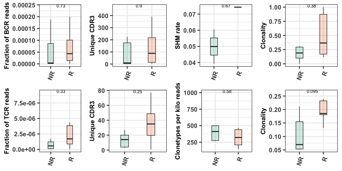
## 8 SRR8281233 IGHM 0.0407 NR6.8 Cohort analysis
The examples above demonstrated the basic immune repertoire-related metrics using a single sample. In the cohort anlysis, all of samples are combined in order to facilitate comparisons within a particular phenotype. The phenotype used for comparison is the one identified in the config.yaml cohort parameter section. This section is described in more detail in Chapter 4.2.1. .
#load the pre-processed results that contain all samples
#These results would be automatically generated after running RIMA immune repertoire module

inputdir <- "TRUST4/Cohort/"
load(paste(inputdir,"TRUST4_BCR_heavy_cluster.Rdata", sep = ""))
load(paste(inputdir,"TRUST4_BCR_heavy_clonality.Rdata", sep = ""))
load(paste(inputdir,"TRUST4_BCR_heavy_SHMRatio.Rdata",sep = ""))
load(paste(inputdir,"TRUST4_BCR_heavy_lib_reads_Infil.Rdata",sep = ""))
load(paste(inputdir,"TRUST4_BCR_Ig_CS.Rdata",sep = ""))
load(paste(inputdir,"TRUST4_BCR_heavy_lib_reads_Infil.Rdata",sep = ""))
load(paste(inputdir,"TRUST4_BCR_heavy.Rdata",sep = ""))
load(paste(inputdir,"TRUST4_TCR_lib_reads_Infil.Rdata",sep = ""))
load(paste(inputdir,"TRUST4_TCR.Rdata",sep = ""))
load(paste(inputdir,"TRUST4_TCR_clonality.Rdata",sep = ""))


#call the ploting function
source("TRUST4/trust4_plot.R")
meta <- read.csv("metasheet.csv")
p <- Trust4_plot(phenotype = "Responder", metasheet = meta)

p